Let’s (no pun intended) look at a set of response times of a web service.

let responseTimes = [ 18.0; 21.0; 41.0; 42.0; 48.0; 50.0; 55.0; 90.0; ] 

People like having a single number to summarize a piece of data. The average is the most popular candidate. The average is calculated by dividing the sum of the input elements by the number of input elements.

let average input =
	let length = input |> Seq.length
	match length with
		| 0 -> raise <| new ArgumentException("Input sequence is empty")
		| _ -> (input |> Seq.sum) / float length 	

// Average = 45.625
// (18 + 21 + 41 + 42 + 48 + 50 + 55 + 90) / 8

The average is a measure of centre which is fragile to outliers; one or two odd irregular values might skew the outcome. The median on the other hand is always representative of the centre, not just when the data distribution is symmetric. The median is determined by sorting the input elements and picking the one in the middle.

let (|Even|Odd|) x =
	if x % 2 = 0 then Even
	else Odd

let median input = 
	let sortedInput = input |> Seq.sort
	let length = input |> Seq.length
	match length with
		| 0 -> raise <| new ArgumentException("Input sequence is empty")
		| 1 -> input |> Seq.nth 0
		| _ -> match length with
			| Even -> ( let first = sortedInput |> Seq.nth (length / 2 - 1)
						let second = sortedInput |> Seq.nth (length / 2)
						(first + second) / float 2)                             
			| Odd -> sortedInput |> Seq.nth ((length - 1) / 2)
				
// Median = 45.0
// 18 21 41 42 48 50 55 90
//          __ __

Both measures are terrible at showing how the data is distributed though. The average and median response time might look fair, but maybe there are a few outliers which are giving a few customers a bad time.

Instead of reducing our input down to a single number, it might be better to extract a table that displays the frequency of various outcomes in the input.

let frequencyDistribution input =
	input |> 
	Seq.groupBy (fun x -> 
		match x with 
		| x when x < 30.0 -> [ 0, 30 ]
		| x when x < 70.0 -> [ 30, 70 ]
		| x when x < 90.0 -> [ 70, 90 ] 
		| _ -> [ 90, System.Int32.MaxValue ] ) |>
	Seq.map (fun (x, y) -> x, y |> Seq.length) 

// Frequency Distribution = seq [
// ([(0, 30)], 2); 
// ([(30, 70)], 5); 
// ([(90, 2147483647)], 1)]

Now this is more useful; we can clearly see that the data is not distributed equally and there are a few outliers in our response times we need to investigate further.

This table takes up quite a bit of ink though. What if we want to get rid of the table, but maintain a feel for the distribution of the data?

The standard deviation measures the amount of variation from the average. A low standard deviation means that the data points are very close to the mean. A high standard deviation indicates that the data points are spread out over a large range of values.
It is calculated by taking the square root of the average of the squared differences of the values from their average value.

let standardDeviation input  =
	let avg = input |> Seq.average
	let x = input |> Seq.map(fun x -> System.Math.Pow(float x - avg, float 2)) |> Seq.sum
	let y = input |> Seq.length |> float
	let variance = x / y
	System.Math.Sqrt variance
	
// Average = 45.625; Standard Deviation = 20.87425148

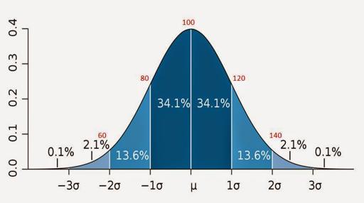
The standard deviation is even more useful when you put the average at the centre of a graph, lay out the input elements according their deviation of the average and see a bell graph drawn. This means that we can use the empirical 68-95-99.7 rule to get a feel of how the data is distributed.

In statistics, the so-called 68–95–99.7 rule is a shorthand used to remember the percentage of values that lie within in a band around the mean in a normal distribution with a width of one, two and three standard deviations, respectively; more accurately, 68.27%, 95.45% and 99.73% of the values lie within one, two and three standard deviations of the mean, respectively. 

For our set of response times, this means that 68.27% of the response times lies within the 24.8 and 66.4 range, 95.45% lies within the 4 and 87.2 range, while 99.73% lies within the -16.8 and 108 range.

When we calculate the standard deviation, we can put one extra number next to the average and derive from just two numbers how the data is distributed.

In conclusion, the mean and the median hide outliers. Looking at the frequency distribution gives you a more complete picture. If we insist on having less data to look at, the standard deviation and the 68–95–99.7 rule can compress the same complete picture into just two numbers.